


Mathematics for an epidemic - Propagation of SARS-CoV-2
During these days of domestic confinement due to the Covid-19 pandemic, the media do not stop offering data and statistics. Those infected are counted by hundreds of thousands and will undoubtedly number in the millions. The number of deceased is predicted to be very high, although in some countries more than others. Some are more scrupulous than others, noting the number of sick and the number of dead. In some nations, appearance weighs more than science and they hide deaths to pretend they have the disease under control. Some politicians are in favour of falsifying the rates of affectation to show social organization, sanitary strength and technical efficiency abroad. Internally, panic is avoided and economic damages are mitigated, as people resign themselves to contagion to safeguard their jobs. Others prefer to be realistic and count cases as strictly as they can to find out what they are doing and thus make sound decisions in order to contain the virus. I think the last attitude is more accurate.
I have read some theories that try to predict the evolution of this disease and I have had time to reflect on the conditions of its spread. I follow the official statistics from the beginning and it has struck me that the data of the cases accumulated up to a date are prioritized over the data of active cases per day. Daily data from many countries where the SARS-CoV-2 virus has spread is collected on a well-known statistical information website, Woldometer. In its graphs, it is observed that the curve that behaves best (in terms of mathematical parameterization refers), is that of the daily active cases.
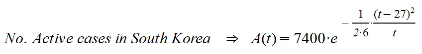
Not all countries, as I said before, have the same reliability, so I focused on those that diagnosed the disease early and took measures to stop it soon after detecting it. One of those countries that has shown the most effectiveness and transparency is South Korea. There it took little time to carry out massive tests to know for sure how the epidemic was spreading. Due to its effectiveness, they took the right measures that made South Korea the first country in the world to contain Covid-19, with a very small margin of affected and deceased.
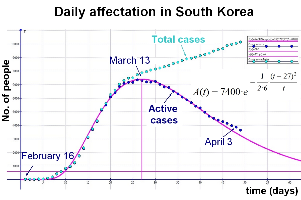
For this reason, I wrote down the data for South Korea and adjusted it to a curve that, by intuition, seemed the most appropriate. I reflected on the variables on which the behavior depends and the consequent analysis was quite adjusted to reality. I kept recording the data daily ... and I didn't have to correct: the graph was still valid day after day.
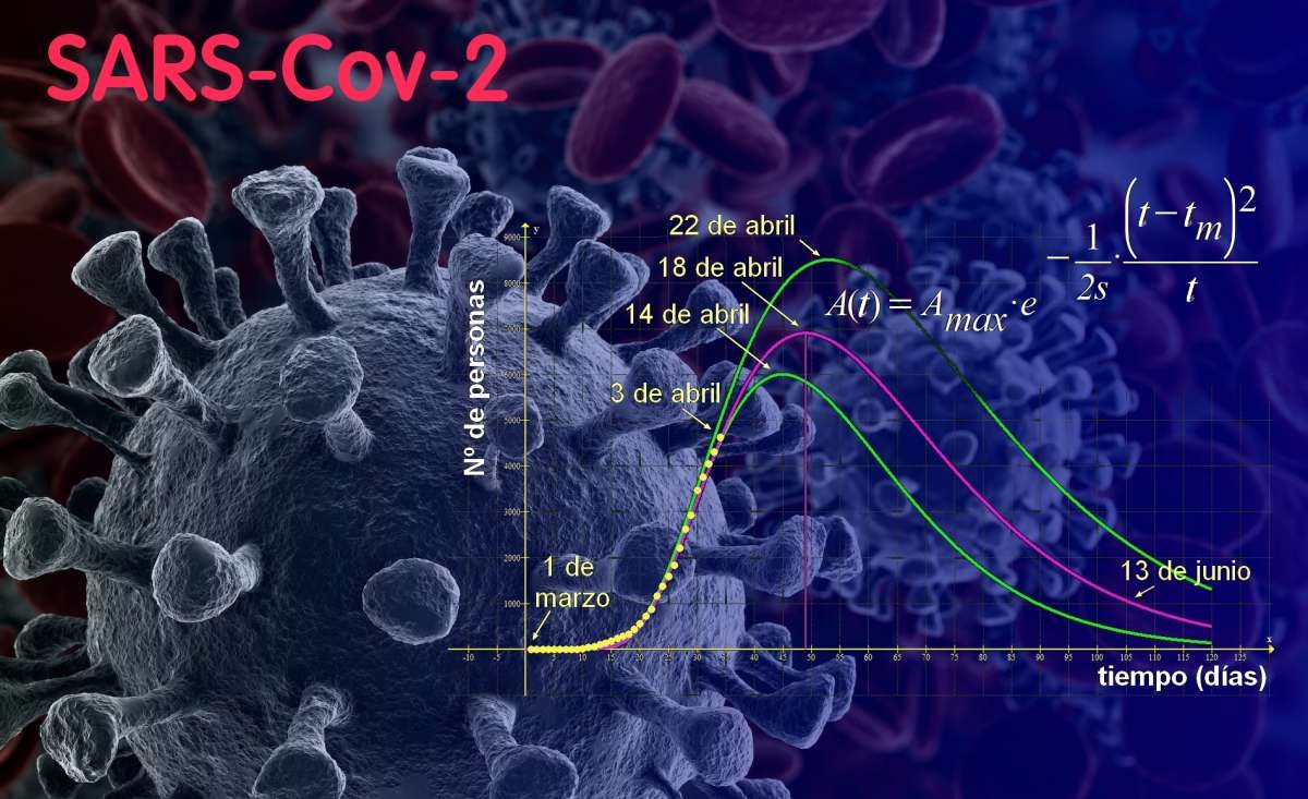
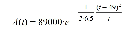
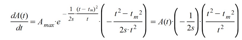
So I started to do the math and I concluded that in all the regions of the world where data is reliably collected, the affected curve fits very well with the following formula:
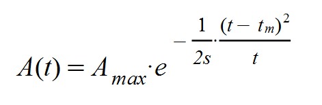
The function A(t) provides the number of people who have the coronavirus each day (the so-called "active cases"), being dependent on the time variable "t". The "Amax" parameter indicates the maximum number of people who have contracted the disease in a day (the famous "peak" for A (t)). The "s" parameter evaluates the transmissibility of the disease and "tm" is the day in which the maximum number of affected "Amax" occurs.
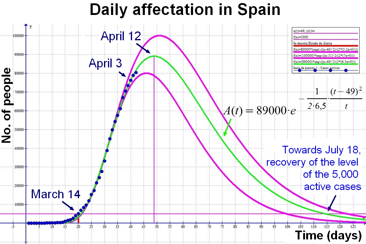
Here is the forecast for Spain:
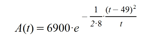
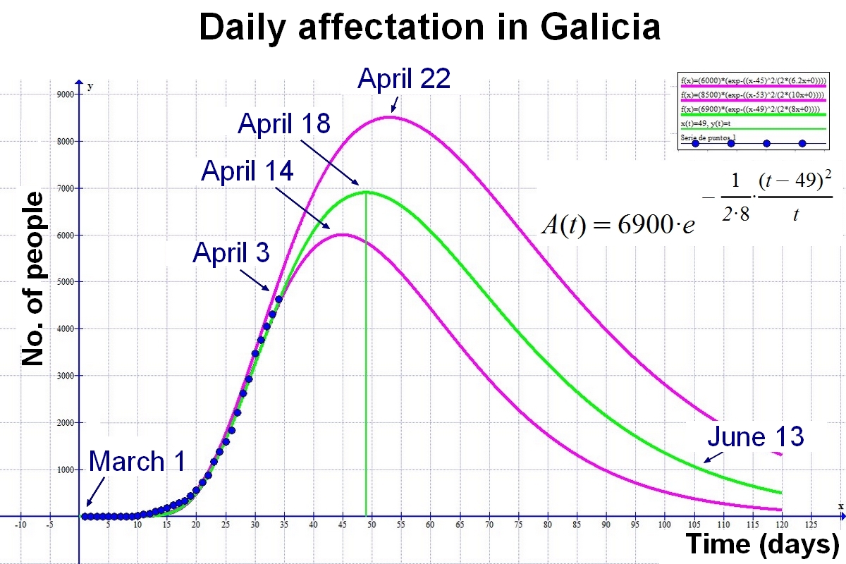
Here is the forecast for Galicia:
Next I will explain the origin of this function.
To start with the analysis, I have assumed a very large population that is only going to be partially infected. There will always be unaffected individuals in significant numbers. I have also considered three remarkable functions in the spread of the disease:
A(t), which is, as I said before, the number of active cases each day.
E(t), which indicates the number of isolated or confined patients.
X(t), indicates the number of total people exposed to the pathogen at each moment.
S(t), which reflects the difference between people susceptible to contracting the disease (or exposed people, less those affected and isolated).
We have assumed that the net amount / quantity of people who are likely to get sick, S(t), are likely to catch it from other unconfined but sick people (with or without symptoms). For this reason I have thought that the following equalities must be met:
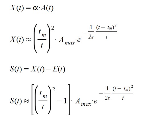
S(t) = X(t) – E(t)
X(t) = α.A(t)
Where "α" is a factor that indicates the proportion between those affected who can transmit the disease and those exposed to it.
E(t) = β.A(t)
Where "β" is a proportionality factor between the real patients who are there and those who are isolated. By assuming β < 1, we are saying that there are patients who are not being considered as such. If β > 1, then we indicate that there are more people considered "sick" than people actually affected. This could happen if we have false positives that are being treated as authentic patients or cured people that are still being counted as active.
S(t) = α.A(t) - β.A(t) = (α - β).A(t)
We have also assumed that the daily variation of those affected is proportional to the number of susceptible people S(t):
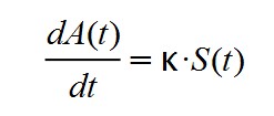
In this way you have to:
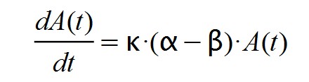
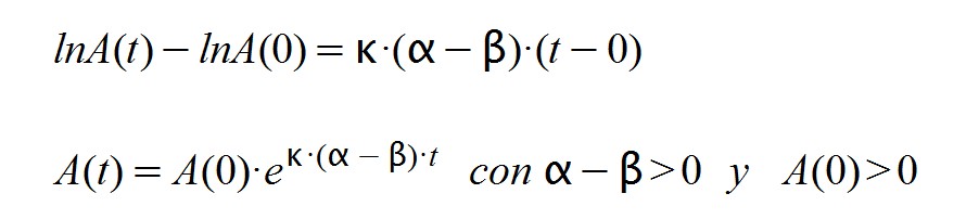
At the beginning of the epidemic it happens that α >> β and, therefore, α – β > 0. If we assume (wrongly) that the factor k.( α – β) remains constant and positive at this stage, we will arrive at the following differential equation:
Whose solution is a growing exponential function, typical of other growth models that occur in nature, such as uncontrolled and unlimited reproduction or nuclear chain reactions.
When the disease has already affected a large population and immunity has been generated, the α and β factors change in such a way that a α < β. This is so because the rate of infection is now less than the cure rate. So:
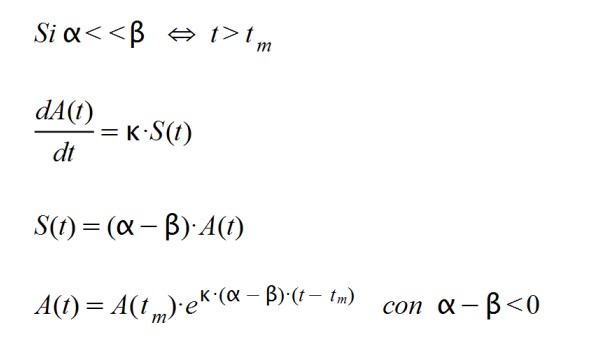
It turns out that A(t) responds in this second case to a decreasing exponential function since its exponent is negative. The time "tm" is the point where the function acquires its maximum value, A(tm) from which it drops to zero.
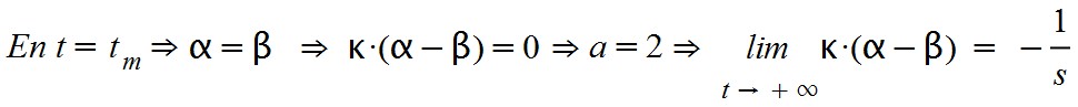
We see clearly that both considerations have to come together if we want to explain the behavior of the current epidemic. The first thing to keep in mind is that the product k.( α – β) must vary with time and go from positive to negative. Just when α = β the product is worth zero. In this case, the function must reach its maximum value (the famous affectation "peak"), since it will turn out that dA(t)/dt = 0.
On the other hand, we know that at time zero the parameter a should tend to infinity, since at that time there are already people who are susceptible to being infected without having registered cases or confined patients.
At t = 0 happens that S(t) = α.A(t) – E(t) > 0, with A(t) = 0 and E(t) = 0.
Another consideration to keep in mind is that the disease must decrease after a certain time since many people will acquire immunity (and some will die), so they are people who will not be able to catch it again. So I thought that there should be a negative factor in the exponential function. I propose it in the following way:
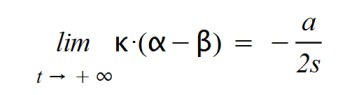
I have chosen this form "–a/2s" for simplification of calculation (and for its meaning), which I will explain later.
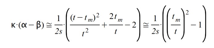
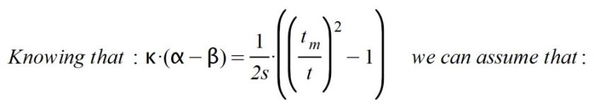
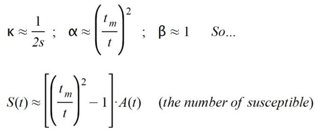
Consequently, as parameterization of the product k.( α – β) I have taken the following approach:
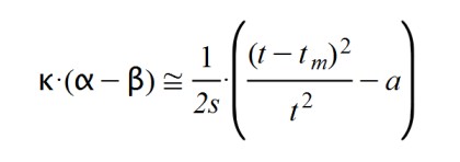
This quadratic form brings together all of the above considerations and is easy to deal with analytically. Earlier I said that:
so that:
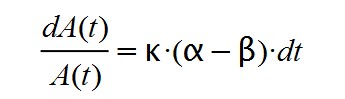
Now we proceed to solve the starting differential equation, that is:
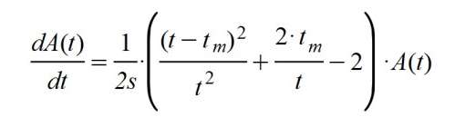
This equation is solved by changing members, as I did previously, the function A (t) and the term dt, and then integrating both parts.
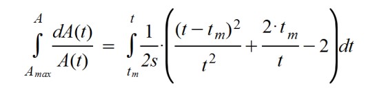
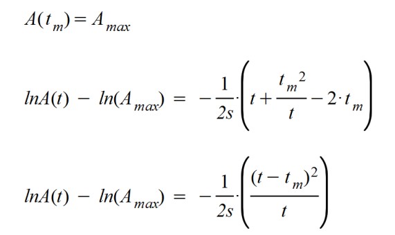
And, as a consequence of the calculation, the initially proposed function is reached. It looks like the typical Gaussian bell ... but with the denominator of the exponent dependent on time, as if the standard deviation of a Gaussian curve increases with time.

As obtained, it appears that the calculation is consistent.
We go one step further in interpreting the function:

On the other hand, it would be nice if we could find out when the "peak" of the curve will happen and how much it opens at the beginning of everything. This would be ideal for taking containment measures and quarantine terms.
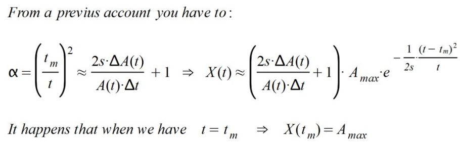
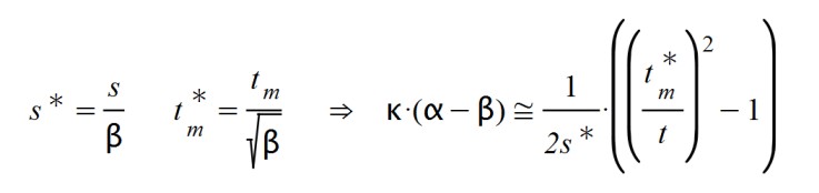
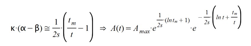
During the first days this will be difficult to guess since there is a lot of variability in the data obtained. As time passes (and as long as data is collected exhaustively), predictions will improve. To guess the maximum point tm, I operate as follows, taking increments instead of differentials, and always as an approximation.
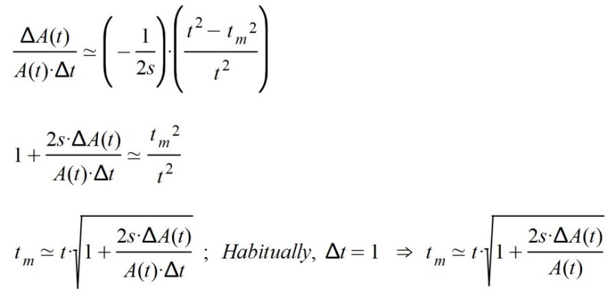
Thus, I have obtained the time in which the maximum of the function A(t) occurs. Now it only remains to adjust two things about it: Amax and s. Both parameters will be adapted according to daily data. It would be nice to have computer software that could do the interpolation properly. I will also say that the official data suffers from systematicity: sometimes they are counted less, other times they change their criteria and, sometimes, "weekend" jumps appear that prevent an effective computer correlation. "Craft" work may be even more suitable than "automatic" work.
I've left the meaning of the "s" parameter unexplained from the start. At this point we have sufficient resources to make sense of this value.
The variable "s" is an always positive number (s > 0); Otherwise it would mean that the epidemic is out of control. It expresses the "weakness" of confinement and other measures that prevent the spread of the epidemic. The higher "s", the weaker the system shows. The higher the "s", the longer it will take to achieve control of the situation and more cases will have to be reported every day.
If we look at the dimensionality of the formula, "s" has been a period of latency or delay, a time when the disease is not attended to. Accordingly, the longer this latency time is, the longer it will take to reach the epidemic maximum.
Since this value is a divisor of the exponent, we understand that it is a very delicate variable to adjust. The number of people affected is very sensitive to this parameter and, therefore, it changes markedly with small variations of "s". Therefore, it is difficult to adjust the function at the beginning of the epidemic: the effectiveness of the social measures that are taken (and that vary in severity over time), have a substantial effect on this variable and, therefore, dramatically influence the long-term function of affected A(t). The uncertainty in the evolution of the epidemic is, therefore, very high in the initial phases of the epidemic.
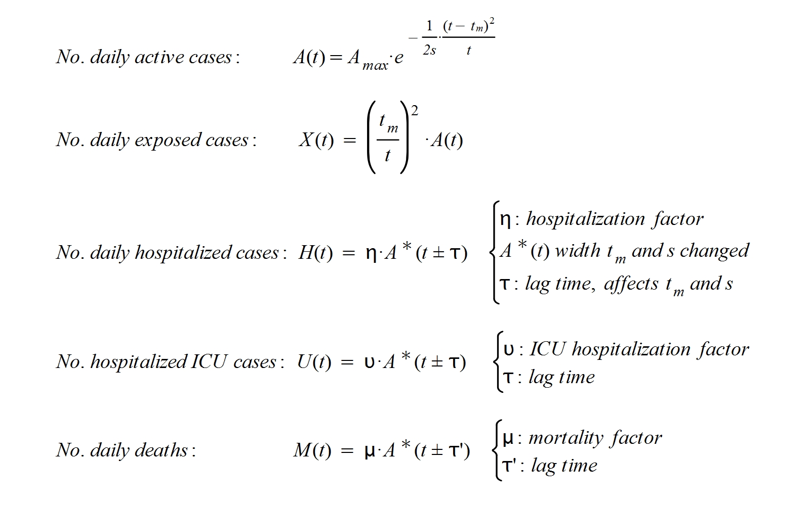
Let us remember that, when knowing the form of A(t), the other quantities presented at the beginning of the calculation can be counted:
With all of the above I am going to consider the special case in which β < 1, that is, E(t) < A(t). This situation occurs when the number of patients treated is less than the number of people active and considered as such. This is equivalent to the fact that there are active people who are not being considered as real patients and, therefore, are not being treated and could be spreading the disease.
We also know that the factor k.(α - β) is inherent to the type of disease because it marks the existing proportion between the variation of the affected cases with respect to the total number of patients affected daily. Remember that:
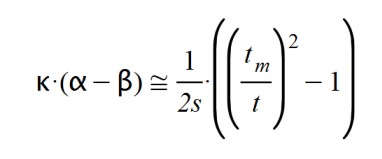
According to this, the disease peak occurs when t = tm, since the parentheses is zero, and the derivative dA(t)/dt is canceled. But this happened if β = 1. What happens if 0 < β < 1 In this case I proceed to simplify expressions and reorder the terms:
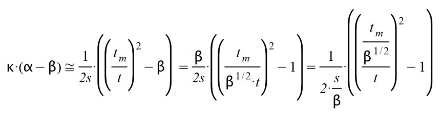
And we get new values for the latency time and the maximum time:
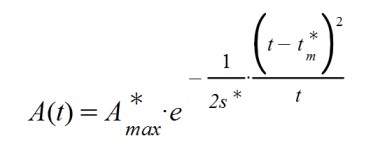
With what we observe two direct alterations in the formula of A(t) and another more indirect one. The effect of decreasing the value of β below unity means that the time to reach the maximum of the curve is amplified.
It also increases the value of latency time, making the effects of the epidemic more lasting. Indirectly we know that the value of Amax will increase, in the number of affected people just at the peak.
Here is a revealing example: if β = 0,5. In this case, the time to reach the maximum is extended by 41% and the latency is double the ideal case (with β = 1). Of course, the number of cases will be dramatically higher, but it is undetermined depending on the severity of the disease (this is the indirect effect).
This reflection leads us to think that there are not many cases of asymptomatic patients that are excluded from the computation. I refer to cases that have not done the PCR tests (or any other test), to find out if they have contracted Covid-19 but if they have it or have had it. So I don't think the infection is as widespread as some say. Rather, I believe that this disease is spreading more in environments where it is in contact with affected cases, that is, in medical centers, nursing homes, prisons and other places of risk due to confinement with high traffic of people.
It would be necessary to calculate X(t) to have a more concrete estimate of the daily number of people who are exposed to the virus.
Here I leave the complementary formulas that complete the study:
There will be a time when the security measures taken in the face of the epidemic (spread according to this model) are relaxed. It is not possible to maintain strict isolation from the population for a long time. So, with a certain probability, there will be a sufficient number of cases that escape from the sanitary control and the people who are not yet immunized will be exposed again. Some of them will contract the disease again and expand it exponentially in a covert manner (more so in this case of SARS-CoV-2, which has a period when the infected person has no symptoms but is contagious).
One of the starting hypotheses was that the majority of the population at the beginning of the epidemic was not immunized. For this reason, and as long as the hypothesis is valid, there will be a recurrence of the epidemic and more or less powerful peaks will occur again.
I consider that this recurrence has a certain monotony if the strict measures are resumed when the new promotions are detected. If we do not resume restrictive measures, we would have dramatic and extensive evolution over time, since this disease has a long period of convalescence. Active cases that develop moderate and severe symptoms take a long time to leave the affected list (at this point we believe that the average is around 30 days).
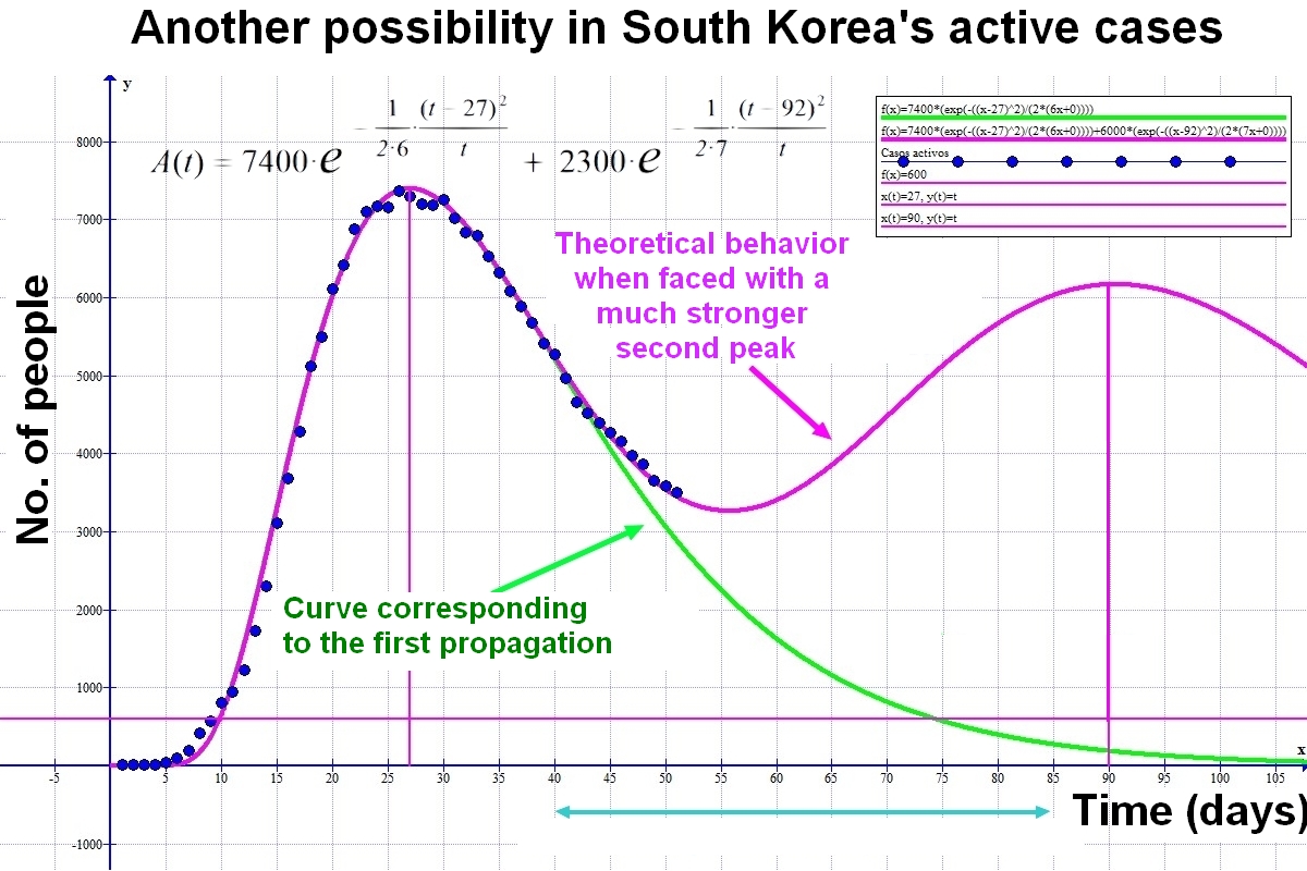
Below is the graph of the possible evolution of the active cases "A(t)" in South Korea
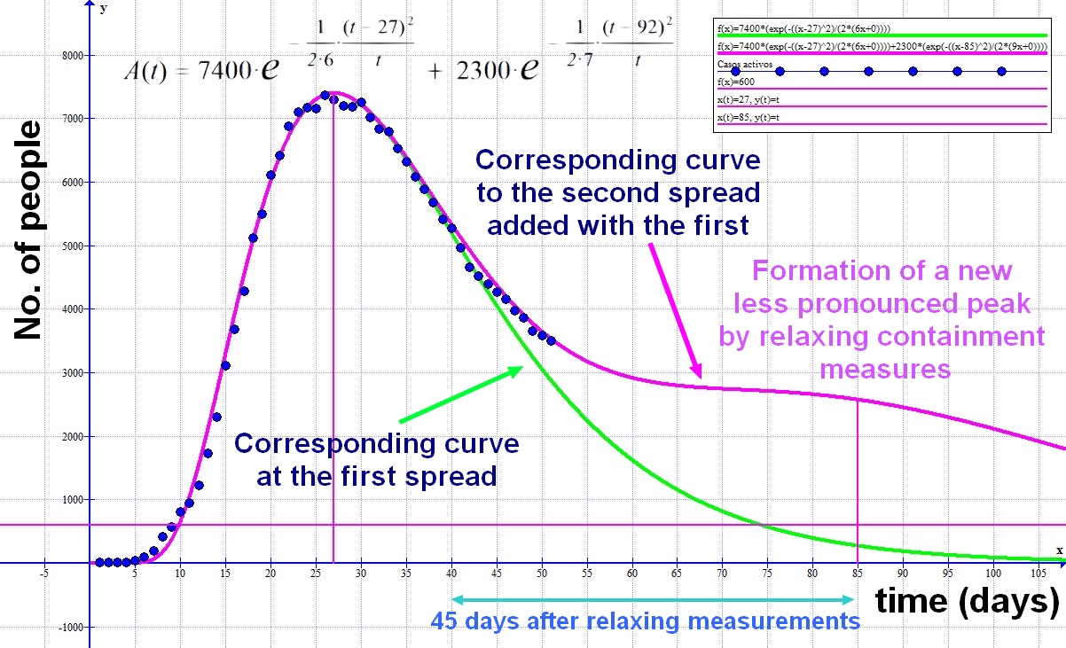
Considering that the first peak occurred after about 45 days, and that the security measures could be moderated 20 days after the maximum, it would be feasible for the next peak to occur 45 days after significantly lifting the containment measures. . This leads to an approximate frequency of 65 days between peaks. As some of the anti-propagation measures will continue to be in force, we will observe that the first curve does not relax as much as expected and that the second enters the count as a stabilization at higher levels than initially expected with a single peak.
If the measurements are even more relaxed we will see how more or less smooth peaks develop over the frequency time that is increasingly difficult to determine. Ultimately, we will have a sustained spread of the epidemic, either until the population is immunized or until a vaccine or other effective system is found to exterminate the pathogen.
Note that the active case function A(x) acts as a soliton wave that can move in time. These types of functions are perfectly summable since their maximum amplitude does not depend on time and the latency parameter s is adaptable. As time passes, the successive peaks increase in width. It seems as if its initial value is gradually increasing. To keep the parameter s proportionally adjusted to each particular situation, its value must evolve asymptotically and decrease according to the expression s~so.t.(1+t2)-1. The different periods that occur may be further parameterized by sums of functions centered on their respective maximum instants in a simple way, only adapting the Amax and s magnitudes for each new case.
NOTE:
There are other possible settings to describe the dependency between dA(t) and A(t), but we have seen that they do not adapt as well to the actual data. On the other hand, their maximum amplitude depends on the moment in which they are produced, making them more difficult to universalize. Be by case:
That it presents a steeper rise at the beginning of the epidemic that does not fit empirical data as well.